Chapter 5 Introduction to Multiple Regression
In the early chapters of our text we observed that everything varies. In a statistical model, the goal is to identify structure in the variation that the data possess. We look to partition the variation in the data into (1) a systematic component, and (2) a non-systematic, or random, component.
In ANOVA testing, the systematic component is comprised of measured factors of research interest that may or may not relate to the response variable. The random component is usually a catch-all for everything else: if the model is built well, there should be no systematic information left in the random component: rather, it should only contain random fluctuations due to the natural inherent variability in the measurements.
Suppose instead of factors (categorical inputs) we have measured predictor variables. For example, consider the admissions data from Chapter 1 of this text; there may be a systematic tendency to see higher freshman GPAs from students with higher ACT scores. Both variables are measured numeric values (compared to pre-determined treatments or categories). This leads to the idea of regression modeling. After this unit, you should be able to
- Recognize the structure of a multiple regression model.
- Fit a regression model in R.
- Interpret the coefficients in a regression model.
- Distinguish between the model constructed in design of experiments (ANOVA) and that in regression.
5.1 Regression Model
The general form of a multiple linear regression (MLR) model is
\[Y = \beta_0 + \beta_1 X_1 + \beta_2 X_2 + \ldots + \beta_k X_k + \varepsilon\] where \(Y\) is the response variable, \(X_j\) is the \(j^\mathrm{th}\) predictor variable with coefficient \(\beta_j\) and \(\varepsilon\) is the unexplained random error. This model is considered linear because the relationship between the predictor variables, and the response is a linear combination. When \(k=1\), the equation reduces to that of a line. When \(k=2\), we are technically modeling a plane in 3-dimensional space and for \(k\geq 3\), the equation defines a hyperplane.
Note that if \(\beta_1=\beta_2=\ldots=\beta_k=0\) we reduce to our baseline model \[Y=\beta_0 + \varepsilon = \mu + \varepsilon\] we saw earlier in the class. The multiple regression model can be considered a generalization of a \(k\) factor ANOVA model but instead of categorical inputs, we have numeric, or quantitative, inputs.
5.1.1 Simple Linear Regression
A special case of the above model occurs when \(k=1\) and the model reduces to \[Y = \beta_0 + \beta_1 X + \varepsilon\]
This is known as the simple linear regression (SLR) model and is covered in most Intro Statistics courses. It is fairly rare that a practicing Statistician will fit a SLR but we will utilize it to explain some key concepts.
It should be noted that multiple regression is in general a \(k + 1\) dimensional problem, so it will usually not be feasible to graphically visualize a fitted model like we can with SLR (which only has 2-dimensions). Even though visualization may not be possible, we can quantitatively explain properties in higher dimensions. In the following sections will we utilize SLR to help visualize important statistical concepts.
The goals of linear regression are:
- Formal assessment of the impact of the predictor variables on the response.
- Prediction of future responses.
These two goals are fundamentally different and may require different techniques to build a model. We outline the fundamental concepts and statistical methods over the next six chapters.
5.2 Fitting a regression model
Regression models are typically estimated through the method of least squares. For the sake of visualizing the concept of least squares, we will consider a SLR example.
5.2.1 Simple Linear Regression Example
Example. Muscle Mass with Age (originally in Kutner et al. (2004)).
A person’s muscle mass is expected to decrease with age.
To explore this relationship in women, a nutritionist randomly selected 15 women from each 10-year age group beginning with age 40 and ending with age 79 and recorded their age (years) and muscle mass (kg).
The data reside in the file musclemass.txt.
The variables in the dataset of interest are mass and age.
First input the data and take a look at the observations.
site <- "https://tjfisher19.github.io/introStatModeling/data/musclemass.txt"
muscle <- read_table(site, col_type=cols())
glimpse(muscle)
## Rows: 60
## Columns: 2
## $ mass <dbl> 106, 106, 97, 113, 96, 119, 92, 112, 92, 102, 107, 107, 102, 115,…
## $ age <dbl> 43, 41, 47, 46, 45, 41, 47, 41, 48, 48, 42, 47, 43, 44, 42, 55, 5…Figure 5.1 displays the data.
ggplot(muscle) +
  geom_point(aes(x=age,y=mass)) +
  labs(title="Muscle Mass vs Age",
       x="Age (years)",
       y="Muscle Mass (kg)") +
  theme_minimal()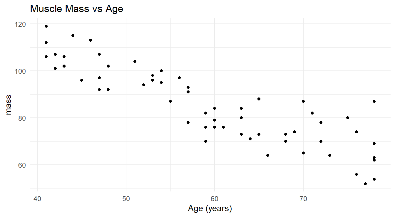
Figure 5.1: Scatterplot showing the relationship between age and muscle mass in a selection of women aged 40 to 79.
We can clearly see the negative trend one would expect: as age increases, muscle mass tends to decrease. You should also notice that it decreases in a roughly linear fashion, so it makes sense to fit a simple linear regression model to this data.
The systematic component of a simple linear regression model passes a straight line through the data in an attempt to explain the linear trend (see Figure 5.2). We can see that such a line effectively explains the trend, but it does not explain it perfectly since the line does not touch all the observed values. The random fluctuations around the trend line are what the \(\varepsilon\) terms account for in the model.
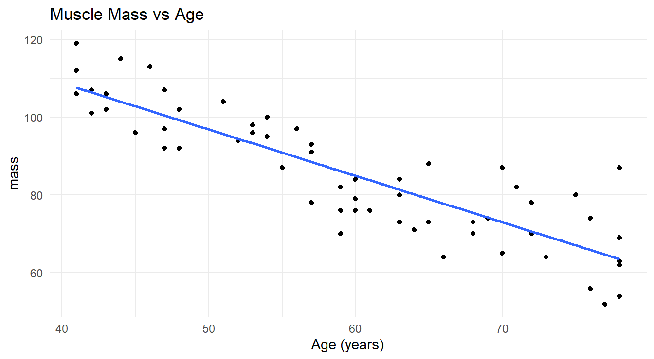
Figure 5.2: Scatterplot showing the relationship between age and muscle mass in a selection of women aged 40 to 79 with a fitted overlayed simple linear regression line.
The next goal is to somehow find the best fitting line for this data. There are an infinite number of possible straight line models of the form \(Y = \beta_0 + \beta_1 X + \varepsilon\) that we could fit to a data set, depending on the values of the slope \(\beta_1\) and y-intercept \(\beta_0\) of the line. Given a scatterplot, how do we determine which slope and y-intercept produces the “best fitting” line for a given data set? Well, first we need to define what we mean by “best”.
Our criterion for finding the best fitting line is rooted in the residuals that the line would produce.
In the two-dimensional simple linear regression case, it is easy to visualize this.
When a straight line is “fit” to a data set, the fitted (or “predicted”) values for each observation fall on the fitted line (see Figure 5.3).
However, the actual observed values randomly scatter around the line.
The vertical discrepancies between the observed and predicted values are the residuals we spoke of earlier.
We can visualize this by zooming into the plot.
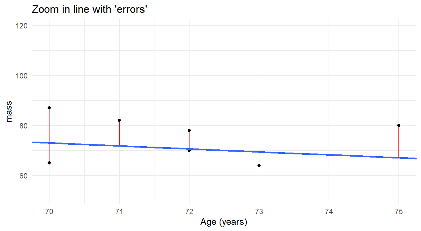
Figure 5.3: Zoomed in view of fitted regression line modeling the relationship of age and mass muscle mass, highlighting the residuals of the fit.
It makes some logical sense to use a criterion that somehow collectively minimizes these residuals, since the best fitting line should be the one that most closely passes through the observed data. We need to estimate \(\beta_0\) and \(\beta_1\) for this “best” line.
Also note in the Figure 5.3 that any reasonable candidate model must pass through the data, producing both positive residuals (actual response values \(>\) fitted response values) and negative residuals (actual response values \(<\) fitted response values). When we collectively assess the residuals, we do not want the positive ones to cancel out or offset the negative ones, so our criterion will be to minimize the sum of squared residuals (thus all are positive). This brings us to what is known as the method of least squares (LS), which is outlined below in the context of simple linear regression.
Method of Least Squares
We propose to “fit” the model \(Y = \beta_0 + \beta_1 X + \varepsilon\) to a data set of \(n\) pairs: \((x_1, y_1), (x_2, y_2), \ldots, (x_n, y_n)\). The goal is to optimally estimate \(\beta_0\) and \(\beta_1\) for the given data.
Denote the estimated values of \(\beta_0\) and \(\beta_1\) by \(b_0\) and \(b_1\), respectively. Note that it is also common to denote the estimated values as \(\hat{\beta}_0\) and \(\hat{\beta}_1\).
The fitted values of \(Y\) are found via the linear equation \(\hat{Y}=b_0 + b_1 X\) (or \(\hat{Y}=\hat{\beta}_0 + \hat{\beta}_1 X\)). In terms of each individual \((x_i, y_i)\) sample observation, the fitted and observed values are found as follows:
\[\begin{array}{c|c} \textrm{Fitted (predicted) values} & \textrm{Observed (actual) values} \\ \hline \hat{y}_1 = b_0 + b_1 x_1 & y_1 = b_0 + b_1 x_1 + e_1 \\ \hat{y}_2 = b_0 + b_1 x_2 & y_2 = b_0 + b_1 x_2 + e_2 \\ \vdots & \vdots \\ \hat{y}_n = b_0 + b_1 x_n & y_n = b_0 + b_1 x_n + e_n \end{array}\]
The difference between each corresponding observed and predicted value is the sample residual for that observation: \[\begin{array}{c} e_1 = y_1 - \hat{y}_1 \\ e_2 = y_2 - \hat{y}_2 \\ \vdots \\ e_n = y_n - \hat{y}_n \end{array}\]
or in general, \(e_i = y_i - \hat{y}_i\). The method of least squares determines \(b_0\) and \(b_1\) so that
\[\textrm{Residual sum of squares (RSS)} = \sum_{i=1}^n e_i^2 = \sum_{i=1}^n\left(y_i - \hat{y}_i\right)^2 = \sum_{i=1}^n\left(y_i - \left(b_0 + b_1 x_i\right)\right)^2\] is a minimum. In other words, any other method of estimating the \(y\)-intercept and slope, \(\beta_0\) and \(\beta_1\), respectively, will produce a larger RSS value than the method of least squares.
Minimizing RSS is a calculus exercise, so we will skip the details here. The resulting line is the “best-fitting” straight line model we could possibly obtain for the data.
- \(b_0\) and \(b_1\) are called the least squares estimates of \(\beta_0\) and \(\beta_1\).
- The line given by \(\hat{Y} = b_0 + b_1 X\) is called the simple linear regression equation.
We use R to fit such models and estimate \(\beta_0\) and \(\beta_1\) using the lm() function (lm=linear model).
No hand calculations required!
Linear models are fit using the R function lm(), and the basic format for a formula is given by response ~ predictor.
The ~ (“tilde”) here is read as “is modeled as a linear function of” and is used to separate the response variable from the predictor variable(s).
For simple linear regression, the form is lm(y ~ x).
In other words, lm(y ~ x) fits the regression model \(Y = \beta_0 + \beta_1 + \varepsilon\).
The \(y\)-intercept is always included, unless you specify otherwise.
lm() creates a model object containing essential information about the fit that we can extract with other R functions.
We illustrate via an example involving the muscle mass dataset.
## List of 12
##  $ coefficients : Named num [1:2] 156.35 -1.19
##   ..- attr(*, "names")= chr [1:2] "(Intercept)" "age"
##  $ residuals    : Named num [1:60] 0.823 -1.557 -3.417 11.393 -6.797 ...
##   ..- attr(*, "names")= chr [1:60] "1" "2" "3" "4" ...
##  $ effects      : Named num [1:60] -658.15 -107.83 -3.34 11.48 -6.69 ...
##   ..- attr(*, "names")= chr [1:60] "(Intercept)" "age" "" "" ...
##  $ rank         : int 2
##  $ fitted.values: Named num [1:60] 105 108 100 102 103 ...
##   ..- attr(*, "names")= chr [1:60] "1" "2" "3" "4" ...
##  $ assign       : int [1:2] 0 1
##  $ qr           :List of 5
##   ..$ qr   : num [1:60, 1:2] -7.746 0.129 0.129 0.129 0.129 ...
##   .. ..- attr(*, "dimnames")=List of 2
##   .. ..- attr(*, "assign")= int [1:2] 0 1
##   ..$ qraux: num [1:2] 1.13 1.19
##   ..$ pivot: int [1:2] 1 2
##   ..$ tol  : num 1e-07
##   ..$ rank : int 2
##   ..- attr(*, "class")= chr "qr"
##  $ df.residual  : int 58
##  $ xlevels      : Named list()
##  $ call         : language lm(formula = mass ~ age, data = muscle)
##  $ terms        :Classes 'terms', 'formula'  language mass ~ age
##   .. ..- attr(*, "variables")= language list(mass, age)
##   .. ..- attr(*, "factors")= int [1:2, 1] 0 1
##   .. .. ..- attr(*, "dimnames")=List of 2
##   .. ..- attr(*, "term.labels")= chr "age"
##   .. ..- attr(*, "order")= int 1
##   .. ..- attr(*, "intercept")= int 1
##   .. ..- attr(*, "response")= int 1
##   .. ..- attr(*, ".Environment")=<environment: R_GlobalEnv>
##   .. ..- attr(*, "predvars")= language list(mass, age)
##   .. ..- attr(*, "dataClasses")= Named chr [1:2] "numeric" "numeric"
##   .. .. ..- attr(*, "names")= chr [1:2] "mass" "age"
##  $ model        :'data.frame':   60 obs. of  2 variables:
##   ..$ mass: num [1:60] 106 106 97 113 96 119 92 112 92 102 ...
##   ..$ age : num [1:60] 43 41 47 46 45 41 47 41 48 48 ...
##   ..- attr(*, "terms")=Classes 'terms', 'formula'  language mass ~ age
##   .. .. ..- attr(*, "variables")= language list(mass, age)
##   .. .. ..- attr(*, "factors")= int [1:2, 1] 0 1
##   .. .. .. ..- attr(*, "dimnames")=List of 2
##   .. .. ..- attr(*, "term.labels")= chr "age"
##   .. .. ..- attr(*, "order")= int 1
##   .. .. ..- attr(*, "intercept")= int 1
##   .. .. ..- attr(*, "response")= int 1
##   .. .. ..- attr(*, ".Environment")=<environment: R_GlobalEnv>
##   .. .. ..- attr(*, "predvars")= language list(mass, age)
##   .. .. ..- attr(*, "dataClasses")= Named chr [1:2] "numeric" "numeric"
##   .. .. .. ..- attr(*, "names")= chr [1:2] "mass" "age"
##  - attr(*, "class")= chr "lm"
You’ll note from the glimpse() function there are many attributes inside the lm object.
We will utilize many of these in our exploration of regression models in the coming chapters.
5.2.2 Multiple Regression Example
To fit a multiple regression, the code is essentially the same. Consider another example.
Example: Property appraisals (example from McClave et al. (2008)).
Suppose a property appraiser wants to model the relationship between the sale price (saleprice) of a residential property and the following three predictor variables:
landvalue- Appraised land value of the property (in $)impvalue- Appraised value of improvements to the property (in $)area- Area of living space on the property (in sq ft)
The data are in the R workspace appraisal.RData in our repository. Lets use R to fit what is known as a “main effects” multiple regression model. The form of this model is given by:
\[\textrm{Sale Price} = \beta_0 + \beta_1(\textrm{Land Area}) + \beta_2(\textrm{Improvement Value}) + \beta_3(\textrm{Area}) + \varepsilon\]
Note the model is just an extension of the simple linear regression model but with three predictor variables. Similar to our study of ANOVA modeling we follow a standard pattern for analysis:
- Describe the data both numerically and graphically.
- Fit a model.
- Once satisfied with the fit, check the regression assumptions.
- Once the assumptions check out, use the model for inference and prediction.
Before embarking on addressing each part, it might be instructive, just once (since this is your first multiple regression encounter), to actually look at the raw data to see its form:
| saleprice | landvalue | impvalue | area |
|---|---|---|---|
| 68900 | 5960 | 44967 | 1873 |
| 48500 | 9000 | 27860 | 928 |
| 55500 | 9500 | 31439 | 1126 |
| 62000 | 10000 | 39592 | 1265 |
| 116500 | 18000 | 72827 | 2214 |
| 45000 | 8500 | 27317 | 912 |
| 38000 | 8000 | 29856 | 899 |
| 83000 | 23000 | 47752 | 1803 |
| 59000 | 8100 | 39117 | 1204 |
| 47500 | 9000 | 29349 | 1725 |
| 40500 | 7300 | 40166 | 1080 |
| 40000 | 8000 | 31679 | 1529 |
| 97000 | 20000 | 58150 | 2455 |
| 45500 | 8000 | 23454 | 1151 |
| 40900 | 8000 | 20897 | 1173 |
| 80000 | 10500 | 56248 | 1960 |
| 56000 | 4000 | 20859 | 1344 |
| 37000 | 4500 | 22610 | 988 |
| 50000 | 3400 | 35948 | 1076 |
| 22400 | 1500 | 5779 | 962 |
We see there are four variables (\(k+1 = 4\)) and 20 observations (\(n = 20\)). Each row contains a different member of the sample (in this case, a different property). Notice the one property with the relatively high selling price as compared to the others.
Pairwise scatterplots are given below to visualize the bivariate associations.
Here we use the ggpairs() function in the add-on package GGally (Schloerke et al., 2018).
Pairwise scatterplots provide a means to visually explore all \(k+1\) dimensions of a dataset, but note that as \(k\) and \(n\) (the sample size) increase, these plots can get very “busy”.
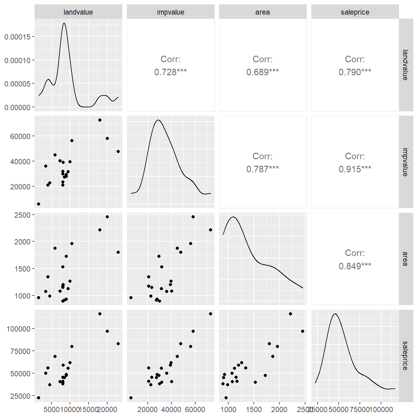
Figure 5.4: Pairs plot showing the relationship between the variables landvalue, impvalue, area and saleprice.
Note that using the columns=c(2:4,1) option, we have reordered the variables for the plot (generally, it is best to have the response variable last so it appears on the \(y\)-axis in the scatterplots).
In the bottom left of the matrix of plots in Figure 5.4 we have pairwise scatterplots.
At first glance, it seems as though each of the three predictors positively relates to sales price.
However, we also get to see the plots of predictors against themselves.
This can be highly informative and will be of some importance to us later on.
There appear to be positive associations between all the predictors (not surprisingly given the context).
It is also instructive to note that three specific individual properties with high appraised land values seem to be the catalyst for these apparent associations.
In the upper right corner of Figure 5.4 are the Pearson correlation coefficients (which measures the amount of linear relationship between the two variables) and along the diagonal are density plots of each variable (providing some information about each variables shape).
We now fit the “main effects” MLR model for predicting \(Y\) = saleprice from the three predictors.
Initially, we might be interested in seeing how individual characteristic(s) impact sales price.
##
## Call:
## lm(formula = saleprice ~ landvalue + impvalue + area, data = appraisal)
##
## Residuals:
##    Min     1Q Median     3Q    Max
## -14688  -2026   1025   2717  15967
##
## Coefficients:
##             Estimate Std. Error t value Pr(>|t|)
## (Intercept) 1384.197   5744.100    0.24   0.8126
## landvalue      0.818      0.512    1.60   0.1294
## impvalue       0.819      0.211    3.89   0.0013 **
## area          13.605      6.569    2.07   0.0549 .
## ---
## Signif. codes:  0 '***' 0.001 '**' 0.01 '*' 0.05 '.' 0.1 ' ' 1
##
## Residual standard error: 7920 on 16 degrees of freedom
## Multiple R-squared:  0.898,  Adjusted R-squared:  0.878
## F-statistic: 46.7 on 3 and 16 DF,  p-value: 3.87e-08
Here are some observations from this regression model fit:
Parameter estimates. The fitted model, where \(Y\) = sale price, is:
\[\hat{Y} = 1384.197 + 0.818(\textrm{Land value}) + 0.819(\textrm{Improvement value}) + 13.605(\textrm{Area})\]
That is, the least squares estimates of the four \(\beta\)-parameters in the model are \(b_0 = 1384.2\), \(b_1 = 0.817\), \(b_2 = 0.819\), and \(b_3 = 13.605\). We will discuss their interpretation later.
Residual standard error. In regression, the error variance \(\sigma^2\) is a measure of the variability of all possible population response \(Y\)-values around their corresponding predicted values as obtained by the true population regression equation. It is called “error” variance because it deals with the difference between true values vs. model-predicted values, and hence can be thought of as measuring the “error” one would incur by making predictions using the model.
Since a variance is always a sum of squares divided by degrees of freedom (SS/df), we can estimate \(\sigma^2\) for a simple linear regression model using the following:
\[S^2_{\varepsilon} = \frac{\sum_{i=1}^n(y_i - \hat{y}_i)^2}{n-p} = \frac{\textrm{RSS}}{n-p}.\]
The degrees of freedom for this error variance estimate is \(n -p\) where \(p\) is the number of parameters estimated in the regression model, here \(p = k+1 = 3+1=4\). So, we had to “spend” \(p=k+1\) degrees of freedom from the \(n\) available degrees of freedom in order to estimate \(\beta_0, \beta_1\), \(\ldots\), \(\beta_k\). (Hopefully you can see that you cannot fit a model with \(n\) or more parameters to a sample of size \(n\); you will have “spent” all your available degrees of freedom, and hence you could not estimate \(\sigma^2\).)
We will usually just denote the estimated error variance using \(S^2\) instead of \(S^2_{\varepsilon}\).
R provides the residual standard error in the summary() output from the linear model fit, which is the square root of the estimated error variance, and thus has the advantage of being in the original units of the response variable \(Y\).
Here, \(s = 7915\) which is our estimate for \(\sigma\).
Applying an Empirical Rule type argument (remember from Intro Statistics!), we could say that approximately 95% of this model’s predicted sale prices would fall within \(\pm 2(7915) = \pm \$15,830\) of the actual sales prices.
The error degrees of freedom are \(n – p\) = \(20 – 4 = 16\).
Interpretation. Since this is essentially the standard deviation of the residuals, we could interpret the value of \(S\) as essentially the average residual size; i.e., the average size of the prediction errors produced by the regression model. In the present context, this translates to stating that the regression model produces predicted sale prices that are, on average, $7,915 dollars off from the actual measured sale price values.
As you can see, such a measure is valuable in helping us determine how well a model performs (i.e., smaller residual error \(\rightarrow\) better fitting model). So, \(S^2\) and the standard errors are important ingredients in the development of inference in regression.
It should also be noted that at this point we are not even sure if this is a good model, and if not, how we might make it better. So later on, we will discuss the “art” of model building.
5.3 Interpreting \(\beta\)-parameter estimates in MLR
Suppose we fit a model to obtain the multiple linear regression equation:
\[\hat{Y} = b_0 + b_1 X_1 + b_2 X_2 + \ldots + b_k X_k\]
What does \(b_1\) mean? In multiple regression involving simultaneous assessments of many predictors, interpretation can become problematic. In certain cases, a \(b_i\) coefficient might represent some real physical constant, but oftentimes the statistical model is just a convenience for representing a more complex reality, so the real meaning of a particular \(b_i\) may not be obvious.
At this point in our trek through statistical model, it is important to remember that there are two methods for obtaining data for analysis: designed experiments and observational studies. It is important to recall the distinction because each type of data results in a different approach to interpreting the \(\beta\)-parameter estimates in in a multiple linear regression model.
5.3.1 Designed experiments
In a designed experiment, the researcher has control over the settings of the predictor variables \(X_1\), \(X_2\), \(\ldots\), \(X_k\). For example, suppose we wish to study several physical exercise regimens and how they impact calorie burn. The experimental units (EUs) are the people we use for the study. We can control some of the predictors such as the amount of time spent exercising or the amount of carbohydrate consumed prior to exercising. Some other predictors might not be controlled but can be measured, such as baseline metabolic variables. Other variables, such as the temperature in the room or the type of exercise done, could be held fixed.
Having control over the conditions in an experiment allows us to make stronger conclusions from the analysis. One important property of a well-designed experiment is called orthogonality. Orthogonality is useful because it allows us to easily interpret the effect one predictor has on the response without regard to any others. For example, orthogonality would permit us to examine the effect of increasing \(X_1\) = time spent exercising on \(Y\) = calorie burn, without any concern for \(X_2\) = carbohydrate consumption. This can only occur in a situation where the predictor settings are judiciously chosen and assigned by the experimenter. Let us look at an example.
5.3.2 Example of Orthogonal Design
Example. Cleaning experiment (from Navidi et al. (2015)).
An experiment was performed to measure the effects of three predictors on the ability of a cleaning solution to remove oil from cloth. The data are in the R workspace cleaningexp.RData. Here are some details:
Response:
pct.removed- Percentage of the oil stain removed
Predictors:
soap.conc- Concentration of soap, in % by weightlauric.acid- Percentage of lauric acid in the solutioncitric.acid- Percentage of citric acid in the solution
Soap concentration was controlled at two levels (15% and 25%), lauric acid at four levels (10%, 20%, 30%, 40%), and citric acid at three levels (10%, 12%, 14%). Each possible combination of the three predictors was tested on five separate stained cloths, for a total of \(5 \times 2 \times 4 \times 3 = 120\) measurements. We want to illustrate the effect of orthogonality on the \(\beta\)-parameter estimates.
load(url("https://tjfisher19.github.io/introStatModeling/data/cleaningexp.RData")
glimpse(cleaningexp)
## Rows: 120
## Columns: 5
## $ soap.conc <int> 15, 15, 15, 15, 15, 15, 15, 15, 15, 15, 15, 15, 15, 15, 15…
## $ lauric.acid <int> 10, 10, 10, 10, 10, 10, 10, 10, 10, 10, 10, 10, 10, 10, 10…
## $ citric.acid <int> 10, 10, 10, 10, 10, 12, 12, 12, 12, 12, 14, 14, 14, 14, 14…
## $ rep <int> 1, 2, 3, 4, 5, 1, 2, 3, 4, 5, 1, 2, 3, 4, 5, 1, 2, 3, 4, 5…
## $ pct.removed <dbl> 20.5, 14.1, 19.1, 20.8, 18.7, 21.2, 22.7, 20.3, 23.9, 20.1…Since we have many numeric levels and we are interested in the numeric association (as compared to the categorical association in ANOVA), we fit a linear model to all three predictors:
##
## Call:
## lm(formula = pct.removed ~ soap.conc + lauric.acid + citric.acid,
##     data = cleaningexp)
##
## Residuals:
##    Min     1Q Median     3Q    Max
## -8.084 -1.995  0.045  2.078  8.787
##
## Coefficients:
##             Estimate Std. Error t value Pr(>|t|)
## (Intercept) -49.6392     2.4169   -20.5   <2e-16 ***
## soap.conc     2.1987     0.0554    39.6   <2e-16 ***
## lauric.acid   0.8629     0.0248    34.8   <2e-16 ***
## citric.acid   2.5956     0.1698    15.3   <2e-16 ***
## ---
## Signif. codes:  0 '***' 0.001 '**' 0.01 '*' 0.05 '.' 0.1 ' ' 1
##
## Residual standard error: 3.04 on 116 degrees of freedom
## Multiple R-squared:  0.963,  Adjusted R-squared:  0.962
## F-statistic: 1.01e+03 on 3 and 116 DF,  p-value: <2e-16
Take note of the model’s \(\beta\)-parameter estimates and their SEs.
Now for illustration only, let’s drop soap.conc from the model:
##
## Call:
## lm(formula = pct.removed ~ lauric.acid + citric.acid, data = cleaningexp)
##
## Residuals:
##    Min     1Q Median     3Q    Max
## -16.15 -11.04  -1.78  11.45  19.78
##
## Coefficients:
##             Estimate Std. Error t value Pr(>|t|)
## (Intercept)  -5.6658     8.1577   -0.69   0.4887
## lauric.acid   0.8629     0.0942    9.16  2.1e-15 ***
## citric.acid   2.5956     0.6449    4.02   0.0001 ***
## ---
## Signif. codes:  0 '***' 0.001 '**' 0.01 '*' 0.05 '.' 0.1 ' ' 1
##
## Residual standard error: 11.5 on 117 degrees of freedom
## Multiple R-squared:  0.461,  Adjusted R-squared:  0.452
## F-statistic: 50.1 on 2 and 117 DF,  p-value: <2e-16
Notice that the coefficient estimates do not change regardless of what other predictors are in the model (this would hold true if we dropped lauric.acid or citric.acid from the model as well - try it!).
This is what orthogonality ensures.
This means that we are safe in assessing the size of the impact of, say, soap concentration on the ability to remove the oil stain, without worrying about how other variables might impact the relationship.
So in a designed experiment with orthogonality properties, we can interpret the value of \(b_1\) unconditionally as follows:
A one-unit increase in \(x_1\) will cause a change of size \(b_1\) in the mean response.
Side note. When we deleted the predictors one at a time, we effectively were taking that predictor’s explanatory contribution to the response and dumping it into the error component of the model. Here, since each predictor was significant (\(p\)-value < 0.0001), this removal caused the residual standard error to increase substantially, which subsequently made the SEs of the coefficients, \(t\)-statistics and \(p\)-values change. We want to make it clear that in practice it is not recommended to remove significant effects from the model — it was only done here to demonstrate that orthogonality ensures that the model’s \(\beta\)-parameter estimates are unchanged regardless of what other predictors are included. However, the results of tests/CIs for those coefficients may change depending on what is included in the model (if you remove an insignificant predictor, the residual SE will change only slightly and hence have negligible impact on SEs of the coefficients, \(t\)-statistics and \(p\)-values).
5.3.3 Observational studies
In most regression settings, you simply collect measurements on predictor and response variables as they naturally occur, without intervention from the data collector. Such data is called observational data.
Interpreting models built on observational data can be challenging. There are many opportunities for error and any conclusions will carry with them substantial unquantifiable uncertainty. Nevertheless, there are many important questions for which only observational data will ever be available. For example, how else would we study something like differences in prevalence of obesity, diabetes and other cardiovascular risk factors between different ethnic groups? Or the effect of socio-economic status on self esteem? It is impossible to design experiments to investigate these since we cannot control variables (or it would be grossly unethical to do so), so we must make the attempt to build good models with observational data in spite of their shortcomings.
In observational studies, establishing causal connections between response and predictor variables is nearly impossible. In the limited scope of a single study, the best one can hope for is to establish associations between predictor variables and response variables. But even this can be difficult due to the uncontrolled nature of observational data. Why? It is because unmeasured and possibly unsuspected “lurking” variables may be the real cause of an observed relationship between response \(Y\) and some predictor \(X_i\). Recall the earlier example where we observed a positive correlation between the heights and mathematical abilities of school children? It turned out that this relationship was really driven by a lurking variable – the age of the child. In this case, the variables height and age are said to be confounded, because for the purpose of predicting math ability in children, they basically measure the same predictive attribute.
In observational studies, it is important to adjust for the effects of possible confounding variables. Unfortunately, one can never be sure that the all relevant confounding variables have been identified. As a result, one must take care in interpreting \(\beta\)-parameter estimates from regression analyses involving observational data.
Here is probably the best way of interpreting a \(\beta\)-parameter estimate (say \(b_1\)) when dealing with observational data:
\(b_1\) measures the effect of a one-unit increase in \(x_1\) on the mean response when all the other (specified) predictors are held constant.
Even this, however, is not perfect. Often in practice, one predictor cannot be changed without changing other predictors. For example, competing species of ground cover in a botanical field study are often negatively correlated, so increasing the amount of cover of one species will likely mean the lowering of cover of the other. In health studies, it is unrealistic to presume that an increase of 1% body fat in an individual would not correlate to changes in other physical characteristics too (e.g., waist circumference).
Furthermore, this interpretation requires the specification of the other variables – so changing which other variables are included in the model may change the interpretation of \(b_1\). Here’s an illustration:
5.3.4 Example of observational regression interpretation
Example: Property appraisals (from McClave et al. (2008)).
We earlier fit a full “main effects” model predicting \(Y\) = salesprice from three predictor variables dealing with property appraisals. This is an observational study, since the predictor values are not set by design by the researcher. Here’s a brief recap of the fitted model:
##
## Call:
## lm(formula = saleprice ~ landvalue + impvalue + area, data = appraisal)
##
## Residuals:
##    Min     1Q Median     3Q    Max
## -14688  -2026   1025   2717  15967
##
## Coefficients:
##             Estimate Std. Error t value Pr(>|t|)
## (Intercept) 1384.197   5744.100    0.24   0.8126
## landvalue      0.818      0.512    1.60   0.1294
## impvalue       0.819      0.211    3.89   0.0013 **
## area          13.605      6.569    2.07   0.0549 .
## ---
## Signif. codes:  0 '***' 0.001 '**' 0.01 '*' 0.05 '.' 0.1 ' ' 1
##
## Residual standard error: 7920 on 16 degrees of freedom
## Multiple R-squared:  0.898,  Adjusted R-squared:  0.878
## F-statistic: 46.7 on 3 and 16 DF,  p-value: 3.87e-08
Interpretation. We see \(b_3\) = 13.605, this value may be best interpreted in context by either of the following:
- “For each additional square foot of living space on a property, we estimate an increase of $13.61 in the mean selling price, holding appraised land and improvement values fixed.”
- “Each additional square foot of living space on a property results in an average increase of $13.61 in the mean selling price, after adjusting for the appraised value of the land and improvements.”
In Summary: When a predictor’s effect on the response variable is assessed in a model that contains other predictor variables, that predictor’s effect is said to be adjusted for the other predictors.
Now, suppose we delete landvalue (an insignificant predictor, \(p\)-value \(>\) 0.05; we will cover this in more detail in the next chapter). How is the model affected?
##
## Call:
## lm(formula = saleprice ~ impvalue + area, data = appraisal)
##
## Residuals:
##    Min     1Q Median     3Q    Max
## -15832  -5200   1260   4642  13836
##
## Coefficients:
##             Estimate Std. Error t value Pr(>|t|)
## (Intercept)  -10.191   5931.634    0.00  0.99865
## impvalue       0.959      0.200    4.79  0.00017 ***
## area          16.492      6.599    2.50  0.02299 *
## ---
## Signif. codes:  0 '***' 0.001 '**' 0.01 '*' 0.05 '.' 0.1 ' ' 1
##
## Residual standard error: 8270 on 17 degrees of freedom
## Multiple R-squared:  0.881,  Adjusted R-squared:  0.867
## F-statistic:   63 on 2 and 17 DF,  p-value: 1.37e-08
Notice that the values of both \(b_2\) and \(b_3\) changed after the predictor \(X_1\) (landvalue) was deleted from the model.
This means that our estimate of the effect that one predictor has on the response depends on what other predictors are in the model (compare this with the example of orthogonality from earlier).
5.4 Why multiple regression?
We briefly tangent with a discussion of why multiple linear regression is superior to running “separate” simple linear regressions.
Because complex natural phenomena are typically impacted by many characteristics, it would be naive in most circumstances to think that just one variable serves as an adequate explanation for an outcome. Instead, we consider the simultaneous impact of potential predictors of interest on the response. Useful models reflect this fact.
The “one-predictor-at-a-time approach” can be quite bad. Suppose you are considering three potential predictors \(X_1\), \(X_2\), \(X_3\) on a response \(Y\). You might be tempted to fit three separate simple linear regression models to each predictor:
\[\begin{array}{c} Y = \beta_0 + \beta_1 X_1 + \varepsilon \\ Y = \beta_0 + \beta_2 X_2 + \varepsilon \\ Y = \beta_0 + \beta_3 X_3 + \varepsilon \end{array}\]
As we shall see, this approach to regression is fundamentally flawed and is to be avoided at all costs. The problem is that if you fit “too simple” a model you will not account for the “collective” impact of multiple predictors of interest, you may then fail to detect significant relationships, or even come to completely wrong conclusions. Below we provide two examples of the dangers of simple linear regression.
To fully understand these examples, you will need to review ??. For now we highlight the individual regression \(t\)-test and residual error to demonstrate the limitations of simple linear regression.
5.4.1 Example of Spurious Correlation
Here is an example to illustrate potential dangers of using a simple linear regression.
Example. Punting Ability in American Football (published in Walpole et al. (2007))
In the game of American Football, a punter will kick a ball to the opposing team as far as possible towards the opponent’s end zone, attempting to maximize the distance the receiving team must advance the ball in order to score. One key feature of a good punt is the “hang time,” the amount of time the ball ‘hangs’ in the air before being caught by the punt returner. An experiment was conducted were each of 13 punters kicked the ball 10 times and the experimenter recorded their average hang time and distances, along with other measures of strength and flexibility.
- Punter_id - an identifier for each punter
- Hang_time - The average hangtim
- Distance -
- RLS - right leg strength (pounds)
- LLS - left leg strength (pounds)
- RHF - right hamstring muscle flexibility (degrees)
- LHF - left hamstring muscle flexibility (degrees)
- Power - Overall leg strength (foot-pounds)
Original Source: Department of Health et al. (1983)
The data is available in the file puntingData.csv.
site <- "https://tjfisher19.github.io/introStatModeling/data/puntingData.csv"
punting <- read_csv(site, col_types=cols() )
glimpse(punting)
## Rows: 13
## Columns: 8
## $ Punter_id <dbl> 1, 2, 3, 4, 5, 6, 7, 8, 9, 10, 11, 12, 13
## $ Hang_time <dbl> 4.75, 4.07, 4.04, 4.18, 4.35, 4.16, 4.43, 3.20, 3.02, 3.64, …
## $ Distance <dbl> 162.50, 144.00, 147.50, 163.50, 192.00, 171.75, 162.00, 104.…
## $ RLS <dbl> 170, 140, 180, 160, 170, 150, 170, 110, 120, 130, 120, 140, …
## $ LLS <dbl> 170, 130, 170, 160, 150, 150, 180, 110, 110, 120, 140, 130, …
## $ RHF <dbl> 106, 92, 93, 103, 104, 101, 108, 86, 90, 85, 89, 92, 95
## $ LHF <dbl> 106, 93, 78, 93, 93, 87, 106, 92, 86, 80, 83, 94, 95
## $ Power <dbl> 240.57, 195.49, 152.99, 197.09, 266.56, 260.56, 219.25, 132.…First note that this data was collected through an experiment, but the data is observational – the experimenter did not control any of the variables of interest.
For our example, we will consider RLS, LLS and Power as potential predictor variables for hang time. Let us look at the scatterplot matrix of the data.
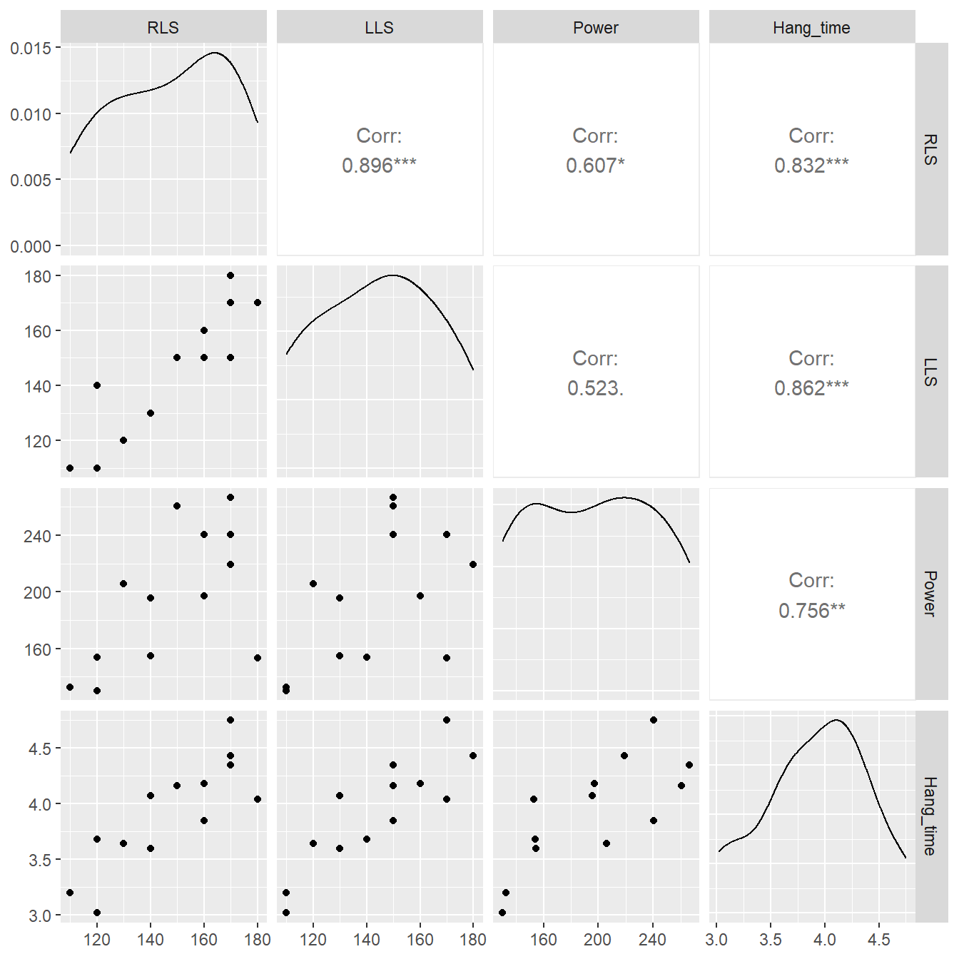
Figure 5.5: Pairs plot showing the relationship between right leg strength, left leg strengh, power and hang time.
Based on Figure 5.5 it appears that all three variables, RLS, LLS and Power, are all moderately or strongly correlated with the hang time. Suppose we fit three simple linear regression models to the data.
slr_rls <- lm(Hang_time ~ RLS, data=punting)
slr_lls <- lm(Hang_time ~ LLS, data=punting)
slr_power <- lm(Hang_time ~ Power, data=punting)
Look at the summary output of each of the three models.
##
## Call:
## lm(formula = Hang_time ~ RLS, data = punting)
##
## Residuals:
##    Min     1Q Median     3Q    Max
## -0.458 -0.183  0.035  0.198  0.431
##
## Coefficients:
##             Estimate Std. Error t value Pr(>|t|)
## (Intercept)  1.28437    0.53569    2.40  0.03538 *
## RLS          0.01785    0.00359    4.98  0.00042 ***
## ---
## Signif. codes:  0 '***' 0.001 '**' 0.01 '*' 0.05 '.' 0.1 ' ' 1
##
## Residual standard error: 0.283 on 11 degrees of freedom
## Multiple R-squared:  0.692,  Adjusted R-squared:  0.664
## F-statistic: 24.8 on 1 and 11 DF, p-value: 0.000419##
## Call:
## lm(formula = Hang_time ~ LLS, data = punting)
##
## Residuals:
## Min 1Q Median 3Q Max
## -0.3616 -0.1701 -0.0662 0.1576 0.4038
##
## Coefficients:
## Estimate Std. Error t value Pr(>|t|)
## (Intercept) 1.27628 0.47390 2.69 0.02091 *
## LLS 0.01838 0.00326 5.65 0.00015 ***
## ---
## Signif. codes: 0 '***' 0.001 '**' 0.01 '*' 0.05 '.' 0.1 ' ' 1
##
## Residual standard error: 0.259 on 11 degrees of freedom
## Multiple R-squared: 0.743, Adjusted R-squared: 0.72
## F-statistic: 31.9 on 1 and 11 DF, p-value: 0.00015##
## Call:
## lm(formula = Hang_time ~ Power, data = punting)
##
## Residuals:
## Min 1Q Median 3Q Max
## -0.4138 -0.2583 0.0003 0.2523 0.4862
##
## Coefficients:
## Estimate Std. Error t value Pr(>|t|)
## (Intercept) 2.40448 0.40679 5.91 0.0001 ***
## Power 0.00773 0.00202 3.83 0.0028 **
## ---
## Signif. codes: 0 '***' 0.001 '**' 0.01 '*' 0.05 '.' 0.1 ' ' 1
##
## Residual standard error: 0.334 on 11 degrees of freedom
## Multiple R-squared: 0.571, Adjusted R-squared: 0.532
## F-statistic: 14.7 on 1 and 11 DF, p-value: 0.0028Although we have not formally covered inference on regression, we might conclude from these results that each of the predictor variables influences hang time (see the very small \(p\)-value associated with the predictor variables). The scatterplots (Figure 5.5) seems to support this as well.
However, it would be erroneous to conclude that this relationship implies causation (a caution wisely applied to all observational data, as we will discuss later). The sample of punters span a range of abilities, and each might utilize their left or right leg more in the act of kicking. So a logical question to ask is “how do all these variables, collectively, influence hang time?”
We fit a multiple regression predicting hang time from all three predictor variables.
##
## Call:
## lm(formula = Hang_time ~ RLS + LLS + Power, data = punting)
##
## Residuals:
##     Min      1Q  Median      3Q     Max
## -0.3463 -0.0832  0.0044  0.0404  0.3412
##
## Coefficients:
##             Estimate Std. Error t value Pr(>|t|)
## (Intercept) 1.103924   0.388267    2.84    0.019 *
## RLS         0.000232   0.006195    0.04    0.971
## LLS         0.013521   0.005744    2.35    0.043 *
## Power       0.004270   0.001540    2.77    0.022 *
## ---
## Signif. codes:  0 '***' 0.001 '**' 0.01 '*' 0.05 '.' 0.1 ' ' 1
##
## Residual standard error: 0.202 on 9 degrees of freedom
## Multiple R-squared:  0.871,  Adjusted R-squared:  0.828
## F-statistic: 20.3 on 3 and 9 DF,  p-value: 0.000241
Compare this result to the simple regression models. When all three variables are included, the variable RLS appears to be unimportant (\(p\)-value = 0.9723). The earlier result occurred because both hang time and RLS are highly correlated with LLS – so the omission of LLS led us to detect what is known as a spurious association between RLS and hang time. To phrase another way, LLS and RLS appear to be providing much of the same, or redundant, information to the model. We may also consider the addition of LLS and Power to be confounding in regards to the variable RLS.
Further, we can see how the multiple regression model improves on the accuracy of the predicted values of the regression model. Consider the table of residual standard errors below.
| Model | Residual.Standard.Error |
|---|---|
| SLR: RLS | 0.283211 |
| SLR: LLS | 0.258640 |
| SLR: Power | 0.334334 |
| MLR: RLS+LLS+Power | 0.202488 |
Note that the multiple regression model has arguably the ‘best’ (smallest) residual standard error of the four models considered – even though it includes the variable RLS which appears to not be important when LLS and Power are included.
The addition of a multiple predictors into the model also alters the nature of the question being asked. The simple linear regression asks: “Does RLS influence hang time?” The multiple linear regression, however, asks a more useful question: “Does RLS influence hang time once any differences due to LHS and Power are considered?” The answer is ‘not really’. It also asks: “Does LLS influence hang time once any differences due to RLS and Power are accounted for?” The answer is ‘yes’.
5.4.2 Example of Confounding in Regression
In the previous section, 5.4.1, we saw how a combination of variables can change the interpretation of a variable in the presence of others. In Section ?? we discussed using blocks as a way to control for potential confounding factors, or nuisance variables. By modeling this extra (in some cases known) variability, we can more accurately determine if the variables of interest influence the response variable. In the below example we demonstrate that regression can be used in a similar way as a block design to control for nuisance variation.
Example. Bleaching Pulp (from Weiss (2012))
The production of paper requires the pupl used in the manufacturing process to be whitened by bleaching in a chemical reaction. The bleaching agents are usually chlorine dioxide (ClO\(_2\)) and hydrogen peroxide (H\(_2\)O\(_2\)). The amounts of these two chemical used in the process effects the whiteness of the pulp, and ultimately that of the paper.
Original source: Zhou (1998)
The file bleachingPulp.txt on the textbook site contains the result of an experiment where 20 combinations of chlorine dioxide and hydrogen peroxide were varied and the brightness or whiteness of the paper was determined (smaller the number, the brighter the paper).
The file is a tabbed separated value format
site <- "https://tjfisher19.github.io/introStatModeling/data/bleachingPulp.txt"
pulp <- read_tsv(site, col_type=cols())
glimpse(pulp)
## Rows: 20
## Columns: 3
## $ ClO2 <dbl> 2.06, 2.06, 2.06, 2.06, 2.06, 3.52, 3.52, 3.52, 3.52, 3.52, …
## $ H2O2 <dbl> 0.0, 0.2, 0.4, 0.6, 0.8, 0.0, 0.2, 0.4, 0.6, 0.8, 0.0, 0.2, …
## $ Whiteness <dbl> 10.55, 9.59, 8.98, 8.46, 7.73, 6.16, 5.55, 5.06, 4.79, 4.74,…Suppose a paper scientist wished to know the effect hydrogen peroxide has on the brightening process. The scientist fits a simple linear regression modeling the whiteness as a function of the amount of hydrogen peroxide.
##
## Call:
## lm(formula = Whiteness ~ H2O2, data = pulp)
##
## Residuals:
##    Min     1Q Median     3Q    Max
## -2.733 -1.756 -0.755  1.179  4.596
##
## Coefficients:
##             Estimate Std. Error t value Pr(>|t|)
## (Intercept)     5.95       1.01    5.91  1.3e-05 ***
## H2O2           -2.06       2.05   -1.00     0.33
## ---
## Signif. codes:  0 '***' 0.001 '**' 0.01 '*' 0.05 '.' 0.1 ' ' 1
##
## Residual standard error: 2.6 on 18 degrees of freedom
## Multiple R-squared:  0.0527, Adjusted R-squared:  7.12e-05
## F-statistic:    1 on 1 and 18 DF,  p-value: 0.33
From the summary output it appears that the amount of hydrogen peroxide does not influence the brightnes of the paper.
Further, we note the residual standard error is 2.59922 which is not all that different than the standard deviation of the Whiteness variable, 2.59931.
However, the above analysis is incorrect because we do not account for the potential effect of the chlorine dioxide (a confounding variable) – the experiment used both. When we fit a multiple regression model we get a different result.
##
## Call:
## lm(formula = Whiteness ~ H2O2 + ClO2, data = pulp)
##
## Residuals:
##     Min      1Q  Median      3Q     Max
## -1.1019 -0.7244 -0.0817  0.6817  1.5107
##
## Coefficients:
##             Estimate Std. Error t value Pr(>|t|)
## (Intercept)   11.939      0.626   19.08  6.4e-13 ***
## H2O2          -2.056      0.712   -2.89     0.01 *
## ClO2          -1.407      0.122  -11.53  1.9e-09 ***
## ---
## Signif. codes:  0 '***' 0.001 '**' 0.01 '*' 0.05 '.' 0.1 ' ' 1
##
## Residual standard error: 0.901 on 17 degrees of freedom
## Multiple R-squared:  0.893,  Adjusted R-squared:  0.88
## F-statistic: 70.6 on 2 and 17 DF,  p-value: 5.83e-09
Based on the multiple regression model, it appears hydrogen peroxide does predict the brightness of the pulp. Also note the decrease in the residual standard error.
For reference, the residual standard error for the simple linear regression with just chlorine dioxide is 1.06879. So it is apparent that both predictor variables provide a better mode than either simple linear regression approach.
5.5 Concluding the Multiple Regression Model
Hopefully the examples outlined in this chapter will give you an appreciation for why we must strive to find a good model for our data, and not fit once and “hope for the best”. In observational studies, many different models may be fit to the same data, but that does not mean they are all good! Findings and results can vary based on which model we choose: precision of our predictions, interpretations of the parameter estimates, etc., so we must use caution and wisdom in our choices. In the following chapters we will cover methods that will help us in our model building.
As statistician George Box once said (Box (1979)):
“All models are wrong but some are useful.”