Chapter 11 Statistical Odds
We now begin our discussion on Generalized Linear Models. But before moving into the specifics of the models, we take a quick tangent to discuss statistical odds. This is necessary in order to truly understand and appreciate the finer details of Logistic Regression.
Consider the game of Roulette:
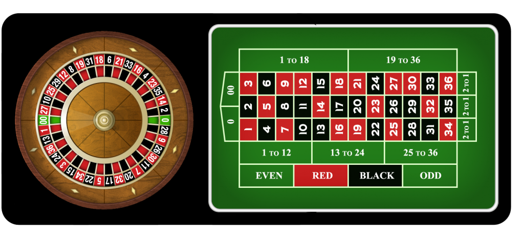
Figure 11.1: Image of American roulette table (with 0 and 00).
In this game a croupier spins the wheel in one direction, then spins a ball, known as the pill, in the opposite direction. The pin will stop on one of the 38 designated numbers (0, 00, 1, 2, \(\ldots\), 36). You will note that zero values are colored green while the remaining numbers alternate the colors red or black. Players of the game will place bets on various parts of the board.
Our goal here is not to study games of chance. However, roulette provides a good example of basic probability and odds. Consider the simple case where the player bets on either red or black.
For discussion, suppose a player places a bet on red. What is the probability they win?
Solution There are 38 possible outcomes in the game, of which 18 are red. The probability the player wins the game is simply 18/38, or 0.4737. The probability the player loses is the complement, which is 20/38 or 0.5263.
11.1 Probability versus Odds
Odds are related to probabilities but are different. The odds of winning are calculated by taking the ratio of the probability of winner the game over the probability of losing the game. Here, that reduces to counting the number of ways you win the game, and divide by the number of ways you lose the game. So in our working example there are 18 ways red occurs while there are 20 ways the outcome is not red. Thus the odds of red are 18/20 = 0.9.
Note, \[ \textrm{Odds of red} = \frac{P(red)}{P(not~red)} = \frac{18/38}{20/38} = \frac{18}{20} = 0.9 = \frac{9}{10}.\]
In the gambling world, one may say the odds of red are 9 to 10. Essentially, there are 9 ways for red to occur for every 10 ways it will not occur.
Thought exercise: For those who like games of chance, in a standard casino betting on red or black typically pays a 1 to 1 ratio, meaning if you bet $100 on black and the outcome is black, you win $100. Should you play this game? Would you play this game?

11.2 Odds ratios
Now that we have a basic understanding of odds, let consider a non-gambling (motivated by data) example.
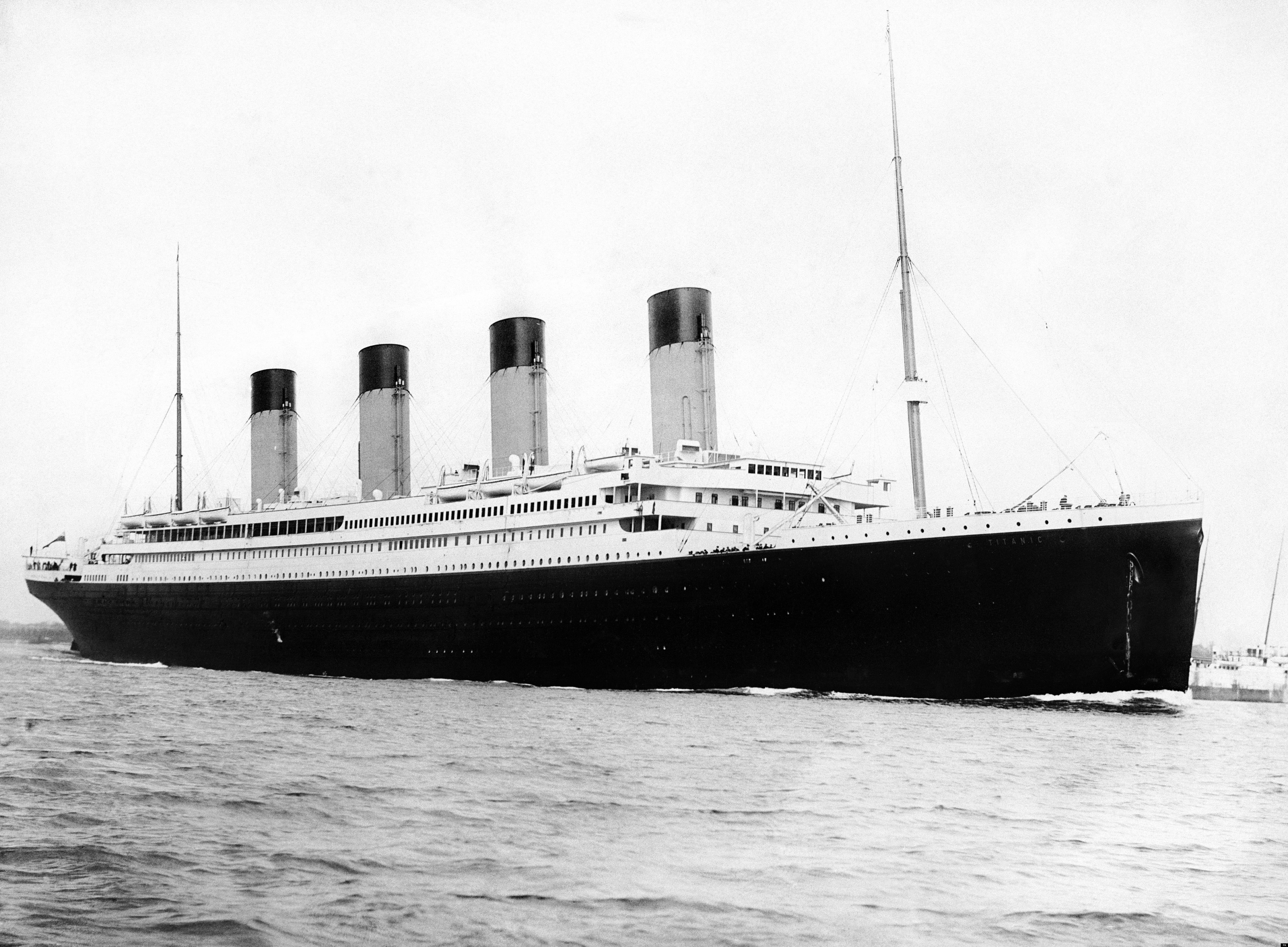
Figure 11.2: Image of the RMS Titanic (damage from iceberg not included)
On April 14, 1912, the RMS Titanic struck an Iceberg in the North Atlantic Ocean off the coast of Newfoundland. Roughly 3 hours after striking the iceberg, the Titanic sunk on April 15, 1912 at 2:20am.
In the paper, The “Unusual Episode” Data Revisited, published in the Journal of Statistics Education vol.3, no.3 (1995), records for 2201 passengers and crew were recorded with their ticket status (the Class variable), Age (categorized as Adult/Child), Gender (Female/Male) and whether they survived the sinking.
##   X Class   Age Gender Survived
## 1 1     1 Adult   Male      Yes
## 2 2     1 Adult   Male      Yes
## 3 3     1 Adult   Male      Yes
## 4 4     1 Adult   Male      Yes
## 5 5     1 Adult   Male      Yes
## 6 6     1 Adult   Male      Yes
In this example, we will explore the odds of surviving the sinking of the Titanic as a function of different variables. First consider the basic case of surviving, we will build a contigency table using the xtabs() function in R.
## Survived
##   No  Yes
## 1490  711
What is the probability a randomly selected passenger suvived the sinking of the Titanic?
For a randomly selected passenger, what are the odds of survival?
Solutions
The probability a randomly selected passenger survived is \(\frac{711}{1490+711}\), or 0.323.
The odds of survival are \(\frac{711}{1490}\) or 0.4772.
Thought exercise: If the odds of Roulette were similar to surviving the Titanic, would you play the game?
In the Titanic dataset we have other information besides whether a person survived or not. Consider a simple question: Does Gender help explain, or predict, a person’s ability to survive this disaster?
We have studied many problems such as this. Does area influence the sale price of a house; does ACT score predict first year GPA; etc…
Here things are different because our response variable (survived or not) is categorical (binary) as well as our predictor variable (gender). The most basic way to explore this sort of relationship is with a two-way contigency table:
##         Survived
## Gender     No  Yes
##   Female  126  344
##   Male   1364  367
If you are a female, what are your odds of surviving?
\(\frac{344}{126}\) = 2.7302
If you are a male, what are your odds of surviving?
\(\frac{367}{1364}\) = 0.2691
Thought exercise – Consider the gambling ideas from above. If you know a person’s gender, are you willing to bet on surviving or not?
It sure looks like there is a relationship, or association, between gender and surviving the sinking of the titanic.
Ultimately in this class we are interested in statistical modeling but the titanic dataset provides an example of categorical data analysis, an area of study that was briefly covered in your Introductory Statistics course. This analysis is still popular in several areas (Psychology and Sociology) and appropriate for some sorts of data.
In the above calculation regarding the Titanic, we essentially are determining an association between categories with a binary response (survived or died). The are several quantitative measures of association for categorical data. There are pros and cons to each. We will just list them here and encourage the interest reader to explore on their own the topic:
- Cramer’s V
- The \(\phi\) statistic
- Relative risk
The first two methods are based on the Chi-square test for association (typically covered in Intro Stat). They can be considered analogous measures of the correlation coefficient \(r\) we saw with regression. Relative risk is derived from the world of Biostatistics and can be a great tool for comparing these sorts of relationships. Basically you compare the conditional probabilities: \(\textrm{P(survived | female)} = \frac{344}{344+126}\) = 0.7319 and \(\textrm{P(survived | male)} = \frac{367}{1731}\) = 0.212
The relative risk of surviving for a female compared to a male is \(\frac{344/470}{367/1731}\) = 3.4522.
If there were no associated between gender and surviving, this relative risk value would be approximately one. Here, we see a random female passenger had greater than a \(3\times\) chance of surviving compared to a male passenger.
Note This example is a bit strange because risk is typically a bad thing. In our above discussion, surviving is the outcome of interest. If I reworked things in terms of not surviving (i.e., death!), we see the relative risk of dying for a female compared to a male is 0.3402. So a randomly selected female would only perish about 1/3 of the rate of a male.
11.3 Ideas of modeling odds
In the above discussion, it sure seems like gender is a predictor for surviving. Other variables are included in the dataset. Some additional contingency table analysis provides additional insight.
##        Survived
## Age       No  Yes
##   Adult 1438  654
##   Child   52   57
The odds of a child surviving are 1.0962 while that of an adult are 0.4548.
Although not ideal, it was better to be a child than an adult on the Titanic.
What about the Class variable. Here things get a little more interesting because there are multiple categories
##       Survived
## Class   No Yes
##   1    122 203
##   2    167 118
##   3    528 178
##   Crew 673 212
We see some obvious things:
- Best to be in first class
- If not first, take your chances in second class.
- Crew members and third class did not fare well.
Of course, all these factors may interact! We’ll revisit that topic in the next chapter but for now we can build more complicated contigency tables. Here we wrap the output of xtabs in the ftable() function for more pleasing output. First consider Class and Age on surviving.
##             Survived  No Yes
## Class Age
## 1     Adult          122 197
##       Child            0   6
## 2     Adult          167  94
##       Child            0  24
## 3     Adult          476 151
##       Child           52  27
## Crew  Adult          673 212
##       Child            0   0
We can see that being a child in first or second class turned out fairly well. The third class children did not survive at as higher of a frequency.
Similarly we can explore other interactions.
##              Survived  No Yes
## Class Gender
## 1     Female            4 141
##       Male            118  62
## 2     Female           13  93
##       Male            154  25
## 3     Female          106  90
##       Male            422  88
## Crew  Female            3  20
## Male 670 192## Survived No Yes
## Age Gender
## Adult Female 109 316
## Male 1329 338
## Child Female 17 28
## Male 35 29Lastly, we can do a full interaction between all the variables
##                    Survived  No Yes
## Class Age   Gender
## 1     Adult Female            4 140
##             Male            118  57
##       Child Female            0   1
##             Male              0   5
## 2     Adult Female           13  80
##             Male            154  14
##       Child Female            0  13
##             Male              0  11
## 3     Adult Female           89  76
##             Male            387  75
##       Child Female           17  14
##             Male             35  13
## Crew  Adult Female            3  20
##             Male            670 192
##       Child Female            0   0
##             Male              0   0
Of note here is the number of 0 counts that occur (all first and second class children survived, and there were no children on the crew). This will impact the feasible choose of models we consider in the next chapter.